Global Change Seminar Summary: Mapping Biodiversity in a Changing World

This post was written by 2019-20 Global Change Fellows, Ana Meza Salazar, Lise Montefiore, and Simon Pinilla Gallego, summarizing the second in the Global Change Seminar series, Mapping Biodiversity in a Changing World, on October 31, 2019.  The discussion was moderated by Global Change Fellow, Simon Pinilla Gallego.
View a recording of the presentation.

---

Panelists:
Dr. Clinton Jenkins, IPE-Instituto de Pesquisas Ecológicas, Brasil
Dr. Krishna Pacifici, Department of Forestry and Environmental Resources, NC State
Dr. Clinton Jenkins
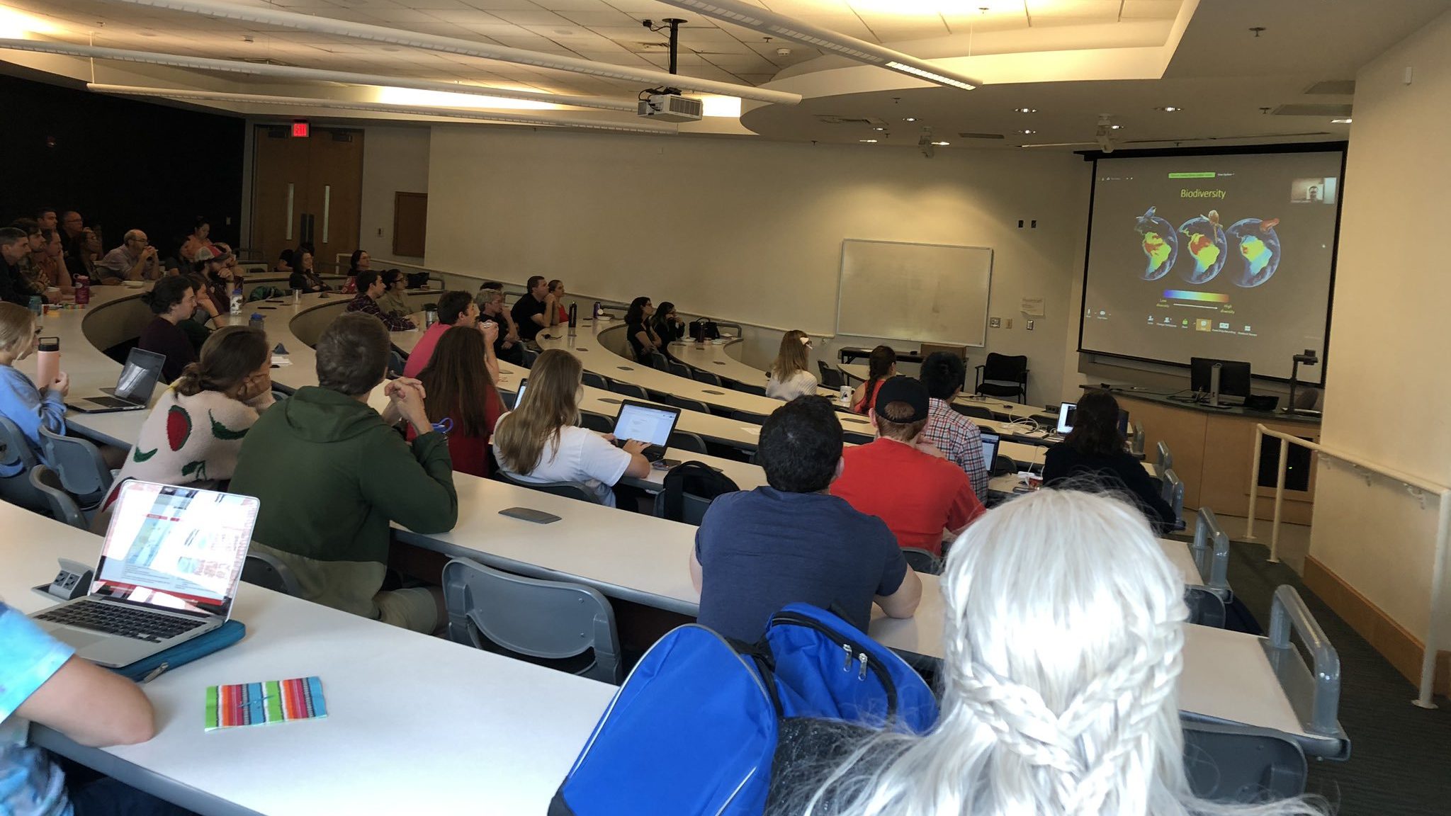
If we take a global view of diversity, we can notice patterns of richness. Dr. Clinton Jenkins displayed a map that synthesizes the distribution of birds, mammals, and amphibians, and illustrated a significant concentration of biodiversity in the north zone of South America. When looking at birds, mammals, and amphibians separately, a similar pattern emerges, but they differ in a few ways. In the Colombian Andes and the Amazon, birds have the highest diversity and mammals show a similar pattern, but amphibians concentrate their diversity in the western part of the Amazon. Though if we take into account the species that have a small range, which represents 50% of bird species, the pattern can change. These small-range birds are concentrated in a particular area, and they are more vulnerable to extinction. The rare species have a high concentration in the Andes, especially in the east. When we look at threatened birds, the pattern looks different. For example, the Atlantic forest of Brazil presents the greatest diversity and this pattern is similar for mammals and amphibians. While the Amazon still conserves about 67% of its vegetation cover, the Atlantic forest has almost completely disappeared, leaving small patches of forest with high fragmentation, threatening biodiversity.
Dr. Jenkins shared a case study in Rio de Janeiro, which he called a brief story of cooperation and restoration. In Rio de Janeiro, 15% of the territory is protected area, and 20 to 25% is forested. In this state, there are more than 700 threatened bird species, making it an area of ​​high conservation interest. The Uniä Biological Reserve (located in Rio de Janeiro) is an area inhabited by threatened species; however, many years ago, it was a fragmented and isolated area that included a gap between forest patches. Although this gap was not very large, it presented a problem for the movement of different animals such as the Golden Lion Tamarin. This primate has shown a recovery in its populations after being part of conservation plans. After several years of negotiation with the owner of this property, the property was purchased, and reforestation plans started with the collaboration of local people and schools. Images of 2007 with the gap and 2018 after reforestation document the species’ recovery, now that they can use all of the forest, with the reserve expanded to cover this territory in order to support the conservation of species.
As for the United States, the maps show a very fragmented territory, where it is necessary to reestablish the connectivity between forests, especially in light of climate change and to anticipate its possible consequences for species. By overlapping biodiversity maps and maps of protected areas, we can create a geographic visualization of areas with high potential for connecting protected areas. Dr. Jenkins proposed that in the future, we should consider climate corridors, rivers, and their connectivity, and also to increase communication of science to the public.
Dr. Krishna Pacifici
Currently, one of the greatest global interests is to understand how biodiversity is going to respond to future changes and stressors. Dr. Krishna Pacifici explained that to map biodiversity, we have to monitor how land use, climate change, invasive species/diseases, overexploitation, and habitat loss are changing over time, and how the species respond to this. When we talk about mapping biodiversity, we have to understand the distribution of species and how are they correlated with the environment, to make models that can explain how the species respond to the environment and make predictions of future responses. In order to understand this, we have to keep in mind two essential elements: how do we use the growing amount of data and how do we account for the change in environmental response?
To model species distribution, we need data with large spatial and temporal extent and data that allows us to understand environmental processes driving geographic distribution, relating observations of a species to environmental characteristics. Much of this information is derived from different sources like academic surveys and citizen science data that have clear advantages like quantity, spatial/temporal coverage, and cost. However, we have to keep in mind the challenges when we use this data, like observation variation, sampling effort, and measurement/recording errors. The question is, what is the best way to use this data to create better biodiversity maps? To answer it, the models take into account the ecological process and observation process. The ecological process include how land uses, climate change, and other covariates influence species occurrence; and the observation process includes how false negatives, false positives, and effort affect the data.
Dr. Pacifici explained the use of those models in two study cases. The first is for a bird called the Brown-headed Nuthatch. For this study, they have data from professional ornithologists (difficult and slow to collect and from limited geographic areas). Also, they have data from amateur ornithologists from citizen science projects (this data is probably less reliable, but it covers a significant geographic area). They developed models that incorporate both datasets and take into account the possible bias and variation. The resulting model is better at generating distribution maps that model with only one of the datasets.
The second case study was developed for the bobcat. Dr. Pacifici pointed out that when we incorporate the effect of disturbance into models, we assume that the effect of the disturbance is the same in all geographic areas, but that is not always true. We can create models that include changes in the effect of the disturbance over time in different geographic areas and use it to create maps of the future distribution of species under specific scenarios. For the bobcat study, they used data from camera traps to model the future distribution of bobcats in North Carolina, taking into account that the effect of housing is different in the three main regions: coastal, piedmont, and mountains.
Overall, the seminar concluded that there is a need for progress in the integration of multiple sources of data for biodiversity mapping. Additionally, accounting for spatial non-stationarity provides robust estimates of environmental relationships with more accurate maps of species distribution, accounts for site-level variation, and reveals variable scales at which species are responding to environmental conditions.